Tutorial and example

Tutorial

The simulation package allows you to compute the secret key rate of a CV-QKD system by giving the parameters of emission, of the channel and of detection.

The parameters of emission are given by choosing a modulation (see here for a list of possible modulations) along with the parameters, including the variance for instance, but also the dimension of discrete modulations when applicable.

The parameters of the channel are given using a channel object, and currently only the qosst_sim.channel.GaussianChannel class is available, and takes as the transmittance and the excess noise as parameters.

Finally the parameters of detection are given using a Detector object (see here for a list of available detectors). For the noisy detector, this include the efficiency and the electronic noise.

Those 3 objects can be fed into one of the simulators, along with some additional parameters. The list of simulators is available here.

Note

One might ask the difference between sim and skr packages. The SKR packages is here to calculate the key rate from the parameters obtained from a real experiment, whereas the sim package will actually generate symbols, and make them follow a simple noise level to then estimate the values of the channel and compute the key rate.

Example

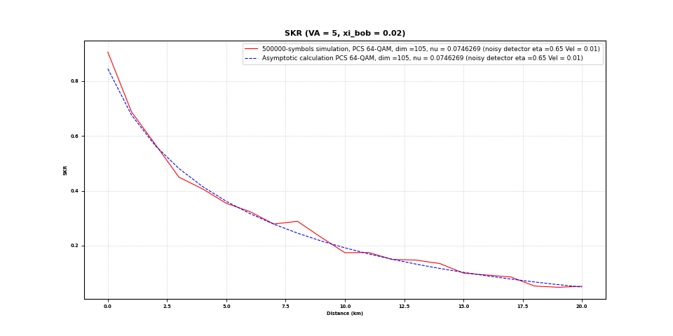
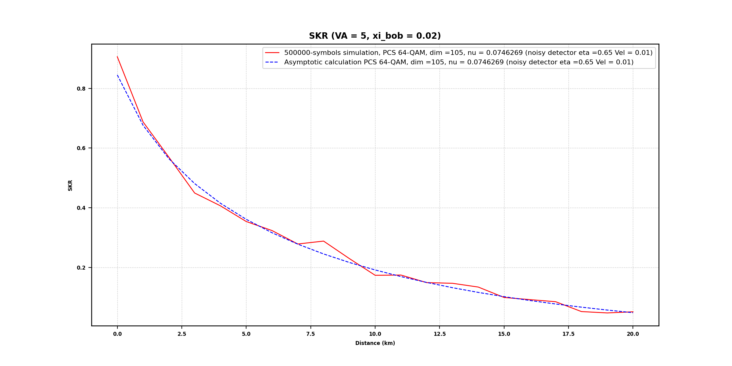
Here below is an example to simulate the key rate for 64-PCSQAM, in asymptotic and finite size scenarios.

from typing import List

import matplotlib.pyplot as plt

from qosst_sim.modulation.gaussian_qam import GaussianQAM
from qosst_sim.detector import NoisyHeterodyneDetector
from qosst_sim.channel import GaussianChannel
from qosst_sim.simulator.finite_size_simulator import FiniteSizeSimulator
from qosst_sim.simulator.gaussian_channel_asymptotic_calculator import (
    GaussianChannelAsymptoticCalculator,
)


def linear_range(start: float, stop: float, num_points: int) -> List[float]:
    """
    Return a linear range from start to stop with num_points.

    Args:
        start (float): start point of the linear range.
        stop (float): end point of the linear range.
        num_points (int): number of points in the range

    Returns:
        List[float]: range.
    """
    step = (stop - start) / num_points
    return [start + x * step for x in range(num_points + 1)]


def transmission(distance: float) -> float:
    """
    Return the transmittance in a fiber with an attenuation coefficient of 0.2dB/km.

    Args:
        distance (float): distance in km.

    Returns:
        float: transmittance in a fiber at 0.2dB/km.
    """
    return 10 ** (-0.02 * distance)


varying_parameter = "Distance (km)"
varying_range = linear_range(0, 20, 20)
beta = 0.95
dim = 105
modulation_size = 8
variance = 5
nu = 0.0746269
num_symbols = 500000
xi_bob = 0.02
electronic_noise = 0.01
eta = 0.65

simulated_skr = []
asymptotic_skr = []


modulation = GaussianQAM(dim, modulation_size, variance, nu)
label = (
    " PCS " + str(modulation_size**2) + "-QAM, dim =" + str(dim) + ", nu = " + str(nu)
)
detector = NoisyHeterodyneDetector(eta, electronic_noise)
label += " (noisy detector eta =" + str(eta) + " Vel = " + str(electronic_noise) + ")"

for distance in varying_range:
    # initialize the channel of the desired type
    transmittance = transmission(distance)
    channel = GaussianChannel(transmittance, xi_bob / (transmittance * detector.eta))

    # initialize the simulator of the desired type
    simulator = FiniteSizeSimulator(modulation, channel, detector, num_symbols, beta)
    calculator = GaussianChannelAsymptoticCalculator(
        modulation, channel, detector, beta
    )

    current_simulated_skr = simulator.skr()
    current_asymptotic_skr = calculator.skr()

    simulated_skr.append(current_simulated_skr)
    asymptotic_skr.append(current_asymptotic_skr)

# plotting tools
_, axes = plt.subplots(figsize=(12, 6))  # plt.subplots(figsize=(12, 6))

for side in axes.spines.keys():  # 'top', 'bottom', 'left', 'right'
    axes.spines[side].set_linewidth(1)

# plotting of the SKR
axes.plot(
    varying_range,
    simulated_skr,
    color="r",
    linestyle="-",
    linewidth=1,
    label=str(num_symbols) + "-symbols simulation," + label,
)
axes.plot(
    varying_range,
    asymptotic_skr,
    color="b",
    linestyle="--",
    linewidth=1,
    label="Asymptotic calculation" + label,
)

title = "SKR (VA = " + str(variance) + ", xi_bob = " + str(xi_bob) + ")"

plt.xlabel(varying_parameter, fontsize=6, fontweight="bold")
plt.ylabel("SKR", fontsize=6, fontweight="bold")
plt.xticks(fontsize=6, fontweight="bold")
plt.yticks(fontsize=6, fontweight="bold")
plt.grid(color="0.8", linestyle="--", linewidth=0.5)

plt.legend(loc="upper right", fontsize=8)

plt.title(title, fontweight="bold", fontsize=10)
plt.show()

(Source code, png, hires.png, pdf)